Monitoring Machine Learning Models Built in Amazon SageMaker
Introduction
Many data science discussions focus on model development. But as any data scientist will tell you, this is only a small—and often relatively quick—part of the data science pipeline. An important, but often overlooked, component of model stewardship is monitoring models once they’ve been released to the wild.
Here we’ll aim to convince any unbelievers that monitoring deployed models is as important as any other task in the data science workflow. For those are already on board with that sentiment, we’ll provide some options to make the process a little less tedious.
Why Monitor Machine Learning Models?
There are a few reasons machine learning models should be tracked once they’ve been deployed. Some are more data science-related, and some are more DevOps concerns.
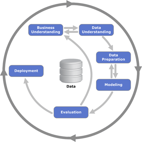
First, ongoing model assessment is a generally accepted best practice. CRISP-DM, a widely-used standard for organizing data science projects, defines a six-phase process for building and deploying analytics work. It devotes an entire phase to model evaluation. In the CRISP-DM standard this evaluation comes before deployment, but its prominence underscores the importance of devoting time to ensuring that models—pre- and post-deployment—meet certain performance criteria.
From a data science perspective, when we evaluate a deployed model, we are usually looking at several things:
- Input data quality
- Distributional characteristics of the input data
- Multivariate relationships of features included in the model
- Model accuracy or loss function results during training phases
- Distributional characteristics of predictions, classifications, and/or parameter estimates
More specifically, since we’ve reviewed all of these pieces in our initial model development, we’re actually looking for changes in any of these items. These types of changes might represent a problem with our input data or model.
From a DevOps perspective, we care about the things DevOps people usually care about: time and cost. Maybe a model runs very quickly on our initial training data, but when dealing with real-world data, it slows down.
The change in model run times might indicate, for example, our training data wasn’t a good match to the real-world data. It also likely translates to increased costs over plan. Regardless of where your machine learning models are hosted (whether in the cloud or on a server rack in your building) CPU time equals money. At a minimum, keeping tabs on the run times for machine learning models helps make for more cost-efficient models applications.
Ongoing monitoring is an important best practice in the data science world, and one of those things that differentiates good organizations from the rest. Although watching something and waiting for it to break is akin to watching paint dry, there are some ways to make the process more fruitful and less tedious. A machine learning framework that automatically generates the most important metrics, such as Amazon SageMaker, as well as a good system for ingesting and reviewing those metrics, can make monitoring models relatively straightforward.
What is SageMaker?
For those who haven’t yet worked with Amazon SageMaker, let’s take a brief detour to discuss what it is and why it exists. Feel free to skip ahead if you are already familiar with SageMaker.
SageMaker is ostensibly a machine learning framework (or PaaS if you prefer), but it can be better described by what it attempts to achieve. At a high level, its primary goal is to make developing and deploying machine learning models less painful, particularly at scale.
One way it does this is by allowing data scientists to apply algorithms to their data in the same ecosystem that stores it. If your organization is already using RedShift or S3 for data storage, SageMaker makes it easy to efficiently extract and analyze that data.
Another way SageMaker simplifies the data science pipeline is by making it very simple to deploy models once they are developed. This step is traditionally handled a number of different ways, and none of them are very good or efficient. SageMaker makes it easy to deploy and dynamically scale a model in single- or low-double-digit lines of code, a vast improvement over traditional options.
Finally, SageMaker makes monitoring deployed models very easy. Each algorithm in SageMaker has a selection of metrics that are produced ‘for free’ with each run. These include standard, cross-validated performance metrics like precision, recall, and MSE, as well as timing and epoch information.
But metrics are only useful if they are looked at, which leads us to…
Frameworks for Monitoring Amazon SageMaker Models
There are a few options for tracking and monitoring metrics produced by SageMaker. The approaches vary in complexity, customization, effort to implement, and ease of use, and can be roughly grouped into three categories:
- Roll Your Own
- AWS-based
- Third-Party Log Analysis Frameworks
Roll Your Own
There are multiple ways to connect to AWS CloudWatch and, once connected, to handle that raw data=. Building your own solution makes sense for organizations that have a custom connection or dashboarding requirements, but those custom solutions are likely to require a good bit of developer time and expertise. Before deciding this is the right approach, it is best to fully evaluate the other two approaches. It is highly likely that one of the options below will be right for most use cases.
AWS-Based
AWS knows its users need easy access to log information. To that end, they have several AWS-based ways to view and analyze logs. SageMaker itself automatically writes some standard machine learning metrics to CloudWatch logs. There are a few methods for accessing those metrics, described here and here. AWS-based metrics may work well for many users, but the charts can be difficult to set up and the system doesn’t have the best UI. If you already have non-AWS logs you need to analyze, using AWS-based machine learning logs also means you have another place to check.
Third-Party Log Analysis Framework
Third-party log collection and analysis frameworks can provide a simpler user interface and reduce the number of places logs are distributed. Although the initial setup may add some time up front, once this is done, a system built specifically to analyze logs is much more likely to be a useful experience.
To show how simple this process can be, we’ll walk through the steps of creating a chart to monitor the training and validation accuracy of an AWS SageMaker model in SolarWinds® Loggly®.
Monitoring SageMaker Models with Loggly
You’ll need four things if you want to follow along with this walkthrough:
- An AWS account with SageMaker configured. Instructions on how to set up your SageMaker account are available here.
- An Amazon SageMaker model. We’ll describe how to set up a toy model below.
- A Loggly account. To create a trial account, follow the steps here.
- A connection between Amazon CloudWatch logs and your Loggly account. We’ll cover this briefly below.
Setting Up a Toy Model
For this walkthrough, we’ll need some model metrics to evaluate. Instead of spending a lot of time working up and explaining a model, we’ll use one of the examples already presented and explained in SageMaker. Follow the steps below to launch the example and run some models.
- After following the steps above to set up your SageMaker account, go to the SageMaker console.
- Create a new notebook instance using the steps listed in this walkthrough. The specifics of the instance aren’t really important for this purpose; you can call it whatever you like and accept the default instance configurations.
- After your instance is created you’ll be taken back to your list of notebook instances, and the instance you just created will now be included. The status will initially be listed as ‘Pending’ as the instance launches, but within a few minutes, it will show as ‘In Service’. Once the instance is in service, click on the ‘Open Jupyter’ link to launch a Jupyter Notebook within the instance.
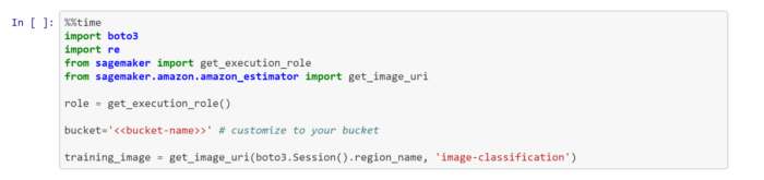
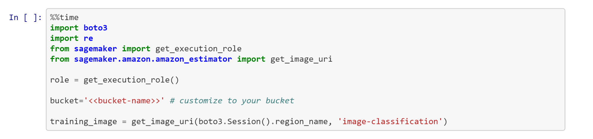
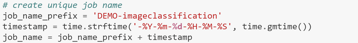
- You now have access to a large list of example notebooks described here (and here). Click the ‘SageMaker Examples’ tab, scroll down to the ‘Introduction to Amazon Algorithms’ section and open the ‘Image Classification’ folder. Find the ‘Image-classification-fulltraining.ipynb’ notebook and click ‘Use’ to open it. Make the changes to the bucket information described in the markdown and cell pictured below, and you are ready to run the algorithm.
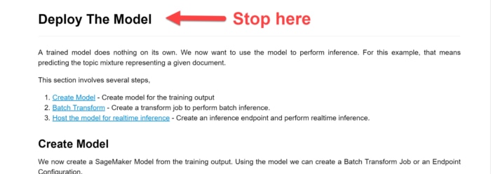
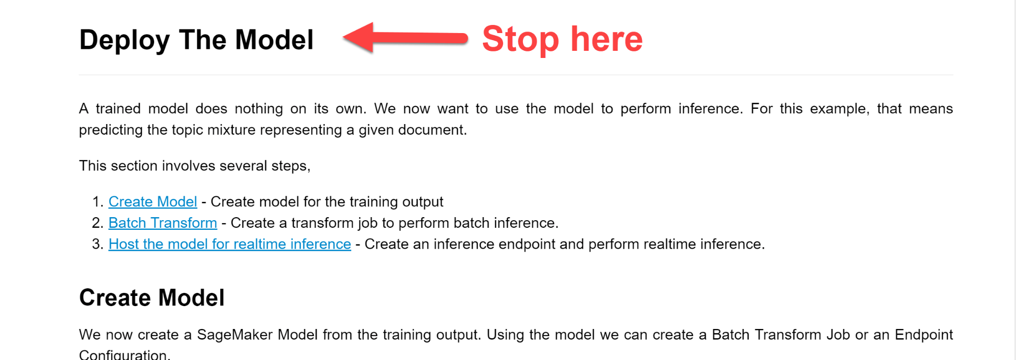
© 2019 Amazon. All rights reserved. - Run all the cells in the notebook down to, but not including, the ‘Deploy the Model’ cell.
© 2019 Amazon. All rights reserved. - Repeat Step 5 again. And again. And again. Run the training steps in Step 5 at least three or four times to generate metrics for a few model runs. In practice, your model runs will likely be automated and if you’re comfortable with Jupyter and Python, it’s fairly easy to combine these cells and wrap the commands in a loop to generate a few models in one click. But if not, that’s perfectly fine. Just manually run the training step a few times. Each run will take about 10 minutes, so this is a good time to kick one off and move on to other things for a bit or get some coffee. If you get a message that the training completed successfully each time, you’re good to go.
A quick sidebar—we’re working with this specific algorithm for a couple of reasons. First, this example requires very little customization to run and it uses an algorithm that automatically generates performance metrics. Second, it takes a while to run, and as we’ll see later, that is useful for this illustration.
Note that because it takes a little while to run (around 10 minutes in the default instance at the time of writing), your AWS account may incur some associated costs. If you’re concerned about cost you can check SageMaker pricing here. As always, make sure to stop your instances when you’re done to prevent unnecessary charges.
Connecting SageMaker and Loggly
By default, SageMaker writes model performance data to CloudWatch. To be able to track our metrics in Loggly, we need to connect the two services. Loggly offers a few ways to do this, but the easiest way is the CloudWatch integration. In fact, all SageMaker model performance metrics go to a special log space called CloudWatch Metrics by default. Since Loggly has a CloudWatch Metrics integration, we’ll use that.
The directions for setting up the integration are covered in detail in the Loggy CloudWatch documention. If you’re not already familiar with connecting CloudWatch and Loggly, you’ll want to set aside some time to get it working.
Displaying Metrics in Loggly
With our accounts and connections all established, we’re ready to start monitoring some models!
Our toy model is a classifier, so we’ll use training and validation accuracy as our performance metrics. In this example use case, we’ll pretend we’re ingesting new data and retraining our model every few minutes (for simplicity, we’ve ignored the prediction step for now). We need to monitor the training and validation accuracy for each of those runs to make sure our model performance meets our minimum criteria, and that we’re not observing anything that would indicate a change in the underlying input data assumptions or overall goodness-of-fit for the model. Above, we ran a few models manually to create some data, but in practice, the data ingestion, model training, and prediction phases would likely be automated.
Verifying the Data
First, let’s verify that we’re seeing our SageMaker data in Loggly. Note that it will take five to ten minutes for your SageMaker data to show up. So if you’ve just finished running the models as described above, now is a good time to take another coffee break or get up and stretch your legs.
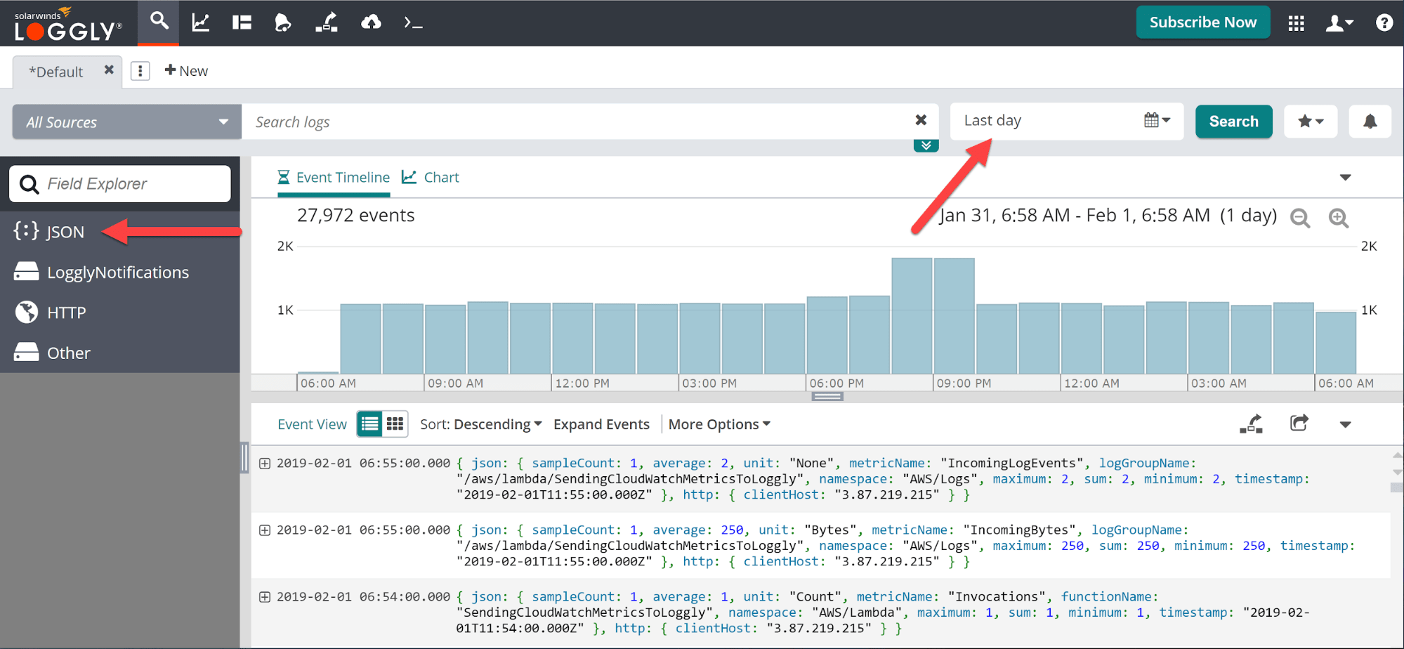
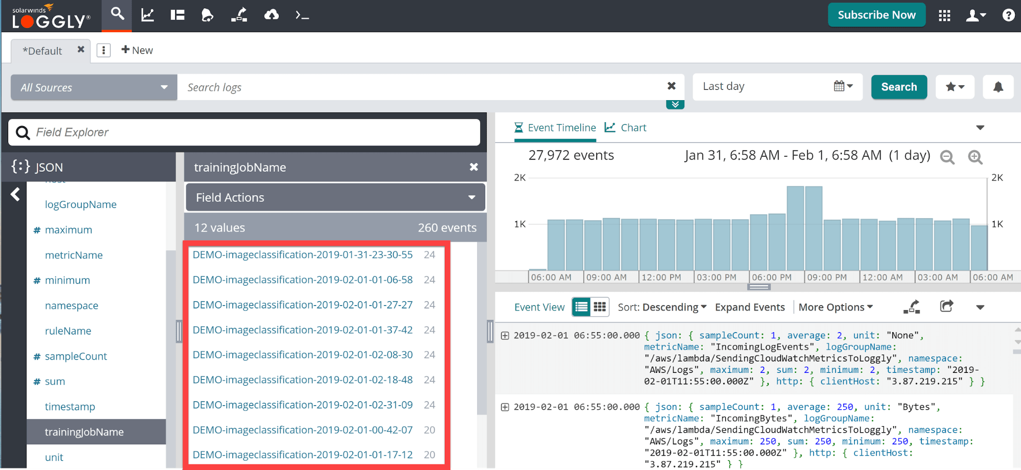
If everything is connected correctly, you should see something like the screenshot above after logging in to Loggly. There are two things to note here. First, if you see event data in the main window, that’s a good sign. If not, first check that your date range (the arrow on the right) covers the appropriate times. If the range is correct but you still don’t see data, you’ll need to go back through the walkthroughs above to make sure all the piping is connected correctly. Second, note the ‘JSON’ tab in the left navigation window. Click there to move on to the next step.
After clicking on the ‘JSON’ menu item, you’ll be given a list of the JSON fields in your data. We’re looking for one field output by our SageMaker models called ‘trainingJobName’.
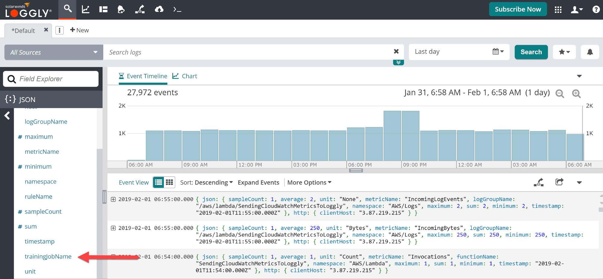
As the field name suggests, this is the unique name given to each of our model runs by this little bit of code in our Jupyter notebook.
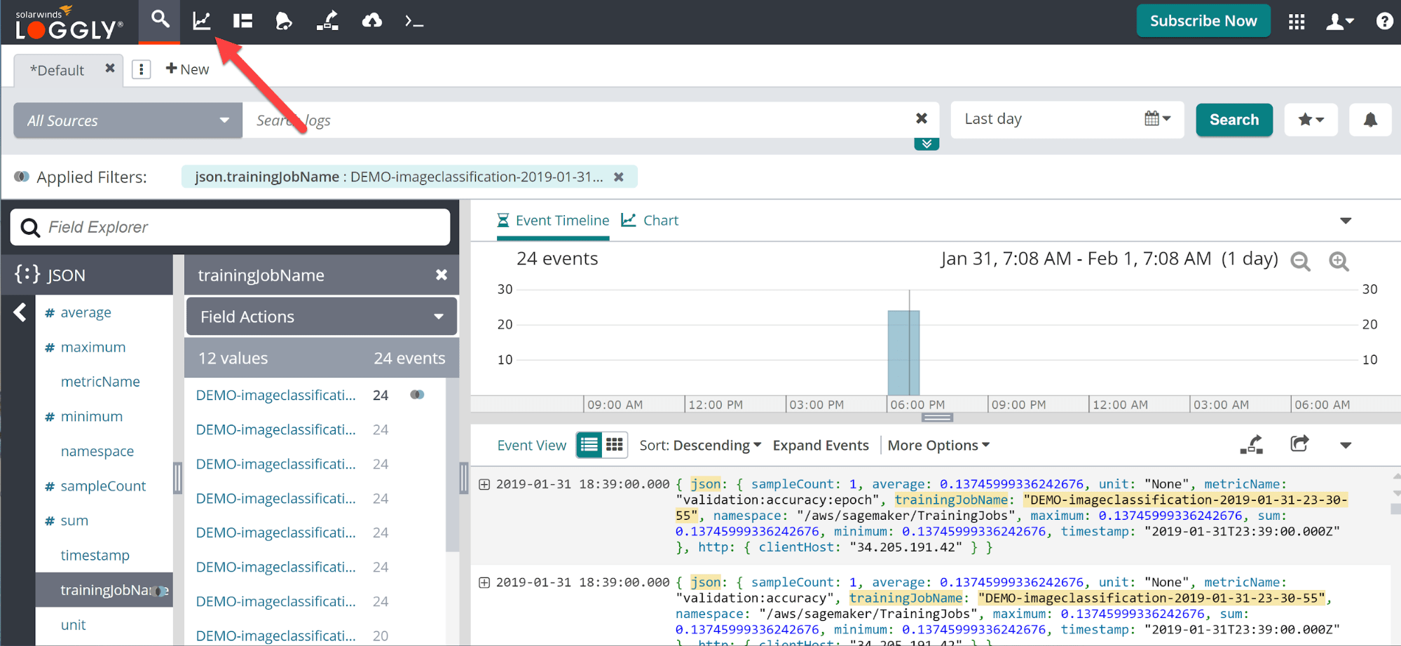
Click on the metric name and you’ll be taken to a list of fields that the element contains. In this case, it is a list of all the models you ran above.
Creating a Chart
Having verified that we have data for our models, we can now create a chart that we can quickly and easily monitor. Click on the ‘Charts’ link on the top navigation menu.
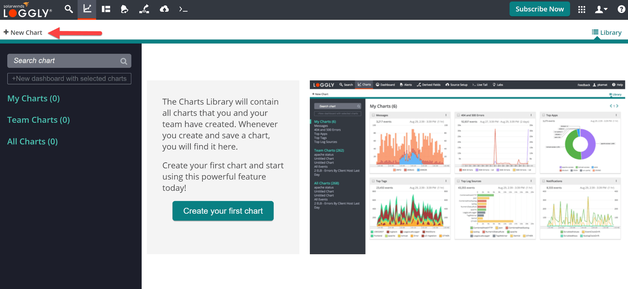
After opening the charts window, click on ‘New Chart’ to add a new chart.
By default, you’ll see a blank chart with the option to customize a few fields and add data for plotting.
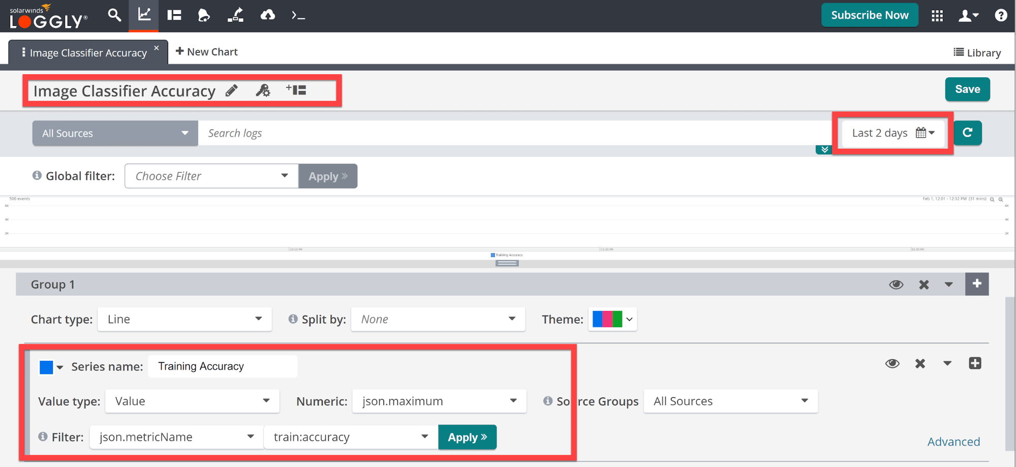
Give your new chart a name to keep things organized. Here I’ve used ‘Image Classifier Accuracy’ since that’s what we’ll be tracking. Check your dates again to make sure that it covers the correct range. If so, scroll down to data Group 1. This is where you will define the data to plot.
The ‘Series name’ field defines how the data is referenced in the legend. This series will plot the training accuracy from our model, so let’s call it ‘Training Accuracy’.
We are pulling a value directly from the JSON fields, so our Value type is ‘Value’. For this metric we only get a single value, so the json.maximum and json.minimum elements are the same; it doesn’t matter which we pick.
We set the filter to ‘json.metricName’ and ‘train:accuracy’ so we’re only plotting the training accuracy data.
Once those changes are made you should see something like the chart below (you can click and drag on the plotted data to have it fill the chart window). You should have a spike (or sawtooth, if you prefer) for every model that you ran.
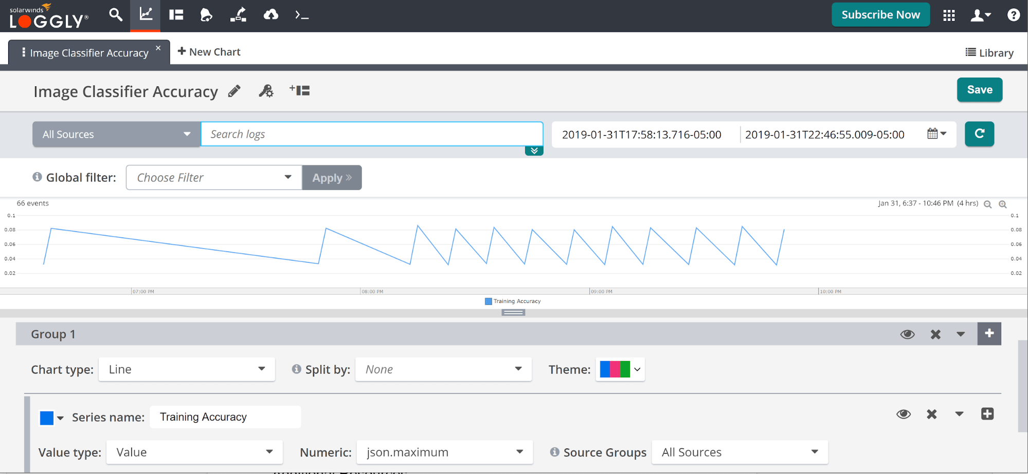
This simple chart only took about five minutes to build and tells us much information about our model performance. The upward slopes are model training runs; the lowest point of the slope tells us the starting accuracy, the highest point tells us the final accuracy, and the width of the slope gives us an indication of the model run time.
The downward slope tells us the length of time between model runs. We can quickly see from the chart above that the model accuracy seems to be consistent across models, but the initial model runs were farther apart than the later runs. In the real world, this might suggest a change in the data ingestion process or some other fluctuation in our automation that we want to review.
Our first series plotted the training accuracy. We can quickly add a series for the validation accuracy by clicking the plus sign (+) to the right of our Training Accuracy series. We’ll name the new series ‘Validation Accuracy’ and keep all the values the same with the exception of changing the second filter item to ‘validation:accuracy’.
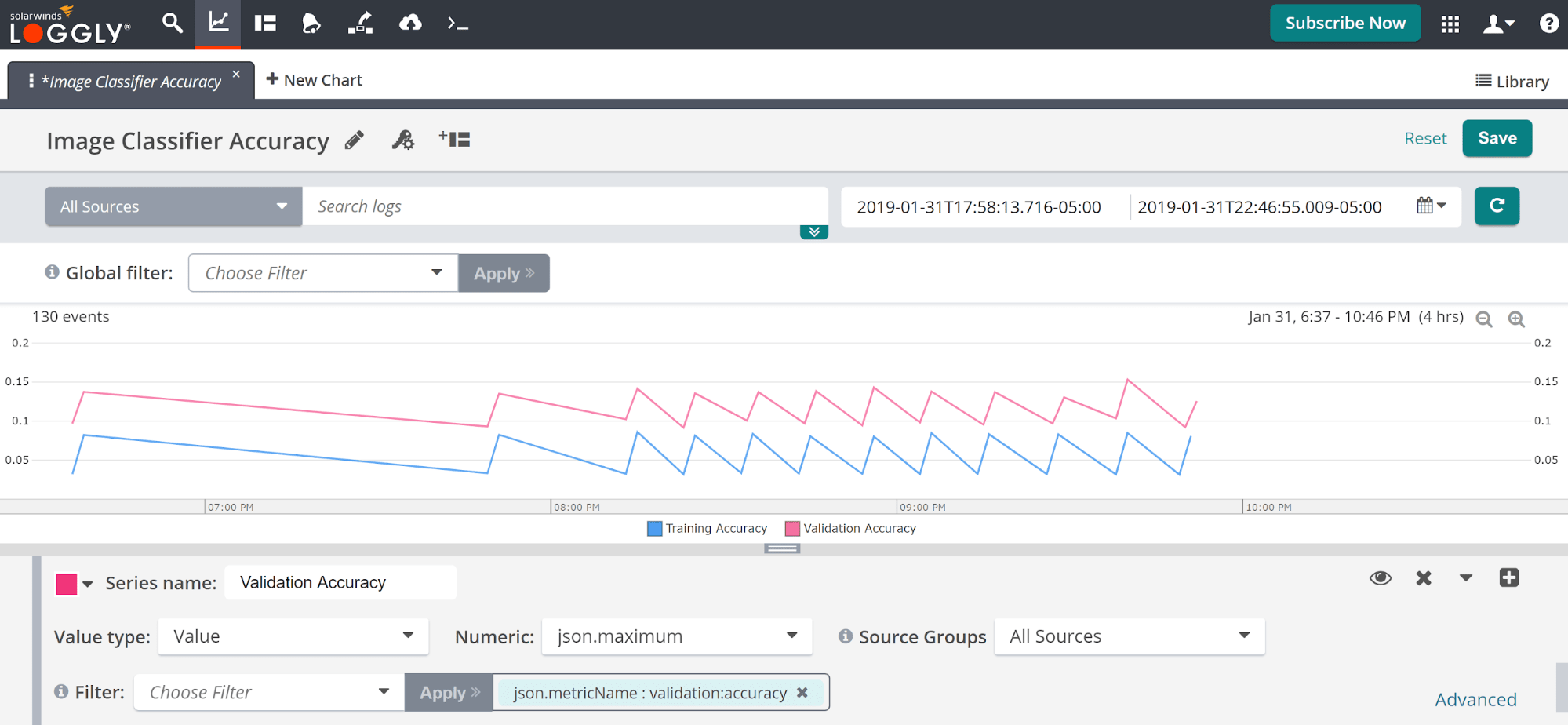
We can now track our validation metrics as well. We see that, for the most part, our validation metrics are consistent with our training metrics and we’re seeing an appropriate relative performance (second sidebar: why is my validation accuracy higher that my training accuracy?). There’s a small dip in the validation performance for our third-to-last training session that is likely due to chance, but we might want to do a deeper dive into that run.
Click ‘Save’ to save the chart. Now this chart can easily be added to a Loggly dashboard alongside any other metrics you want to review.
Summary and Next Steps
In this post, we covered some important reasons to monitor machine learning models. Not only is monitoring your models a good best practice, but it also helps avoid those nightmare scenarios where organizations discover a model has been broken for three months (or running at twice the original cost) and no one realized.
We covered some of the alternatives for monitoring metrics generated by one of the most popular cloud-based machine learning frameworks, Amazon SageMaker. SageMaker has been developed with monitoring in mind, so it makes generating and pulling metrics relatively painless.
Finally, we showed how to use a robust, full-featured log monitoring service (i.e., Loggly) to quickly build charts that make it simple to monitor your models.
To get started with SageMaker, you can begin setting up your account here. If you don’t already have a SolarWinds Loggly account, you can easily get one started here.
The Loggly and SolarWinds trademarks, service marks, and logos are the exclusive property of SolarWinds Worldwide, LLC or its affiliates. All other trademarks are the property of their respective owners.

Loggly Team