In the first two parts of this series on how Loggly uses Loggly, we looked at gathering and structuring data to help us solve the problem of indexing hotspots in our Elasticsearch clusters. Now it’s time for the rubber to hit the road. Let’s take this big data out for a spin with Loggly!

Oh no! A Kafka spike!

Early one morning, a member of our on-call team was paged about a Kafka delta for one of our clusters that had exceeded our alert threshold (2GB). When we looked at the system, we discovered that one of our two writers was not consuming from the Kafka queue, even though the writer process itself was still active. We restarted the writers and saw a rapid recovery in the delta.

If we look at the Kafka deltas for a period of about six hours before and after this, we can clearly see the increase:

Diving in to +/- three hours, we see more detail:

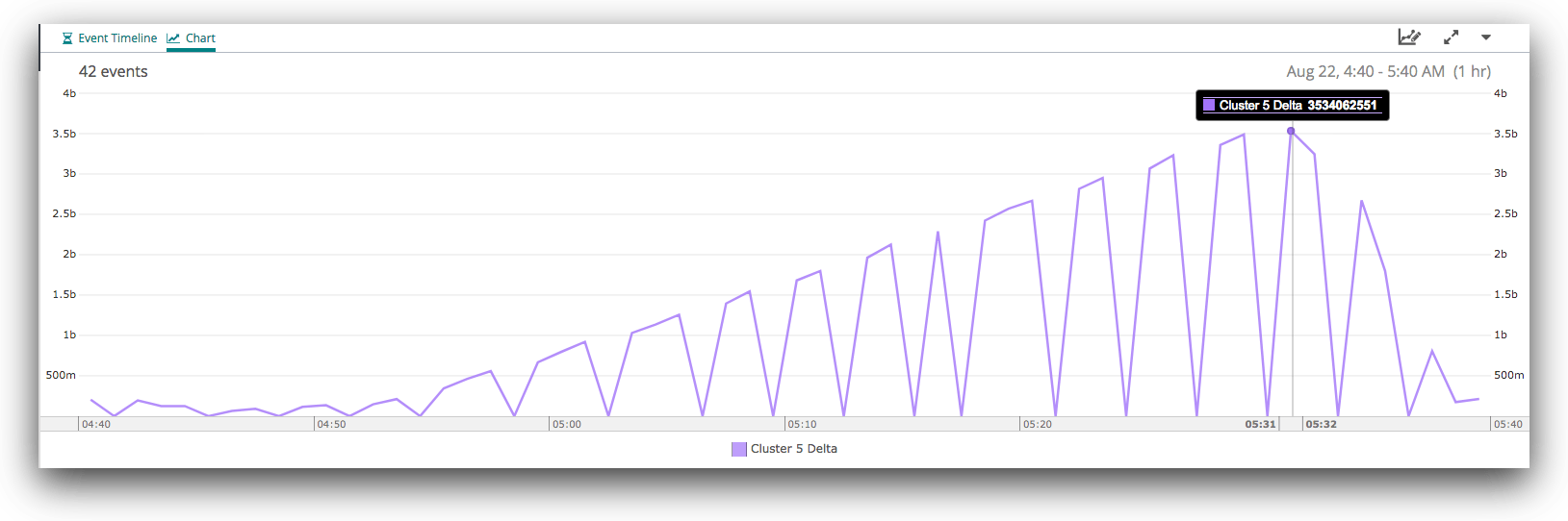
Finally, if we zoom all the way in, we can see the gradual increase in the delta from around 04:55 to its peak at 05:31, and then the rapid recovery, which was complete by 05:38.

What were the writers doing?

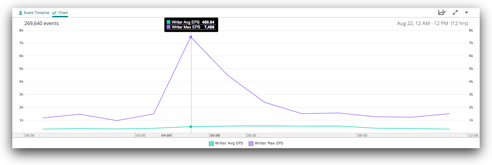
Let’s now see what the writers were doing during this time. At the 12-hour level, we see a similar spike:

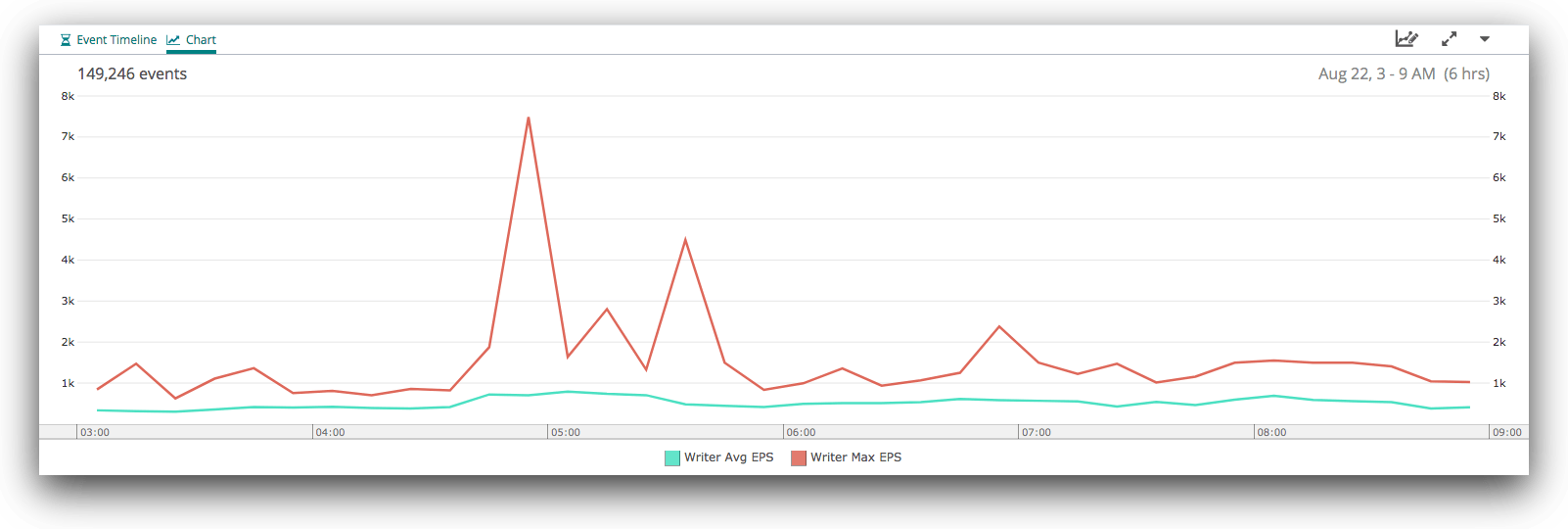
When we zoom in to six hours, we see a more complex pattern, with a major spike just before 05:00, then some instability before things mostly level out around 06:00. There are a few lumps and bumps after that, but nothing terribly unusual.

Zooming in further, and splitting by process ID, we can see the source of the three spikes from around 04:30 to 06:00:

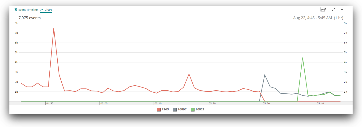
Remember that rogue writer that was not consuming from Kafka? It was also not logging its metrics, so we can only see the performance of the other writer here—the red line. When we restarted the writers, we staggered the restarts. The first was started at 05:30 (the blue line), followed by the second at 05:37. We can see both spike immediately after startup, then quickly fall back into their normal indexing performance. The spike after startup shows that they were running at full speed to clear the backlog in the Kafka queue.

Are our indices balanced?

Does our _cat/shard logging give us any more insight into what’s going on? Let’s take a look…

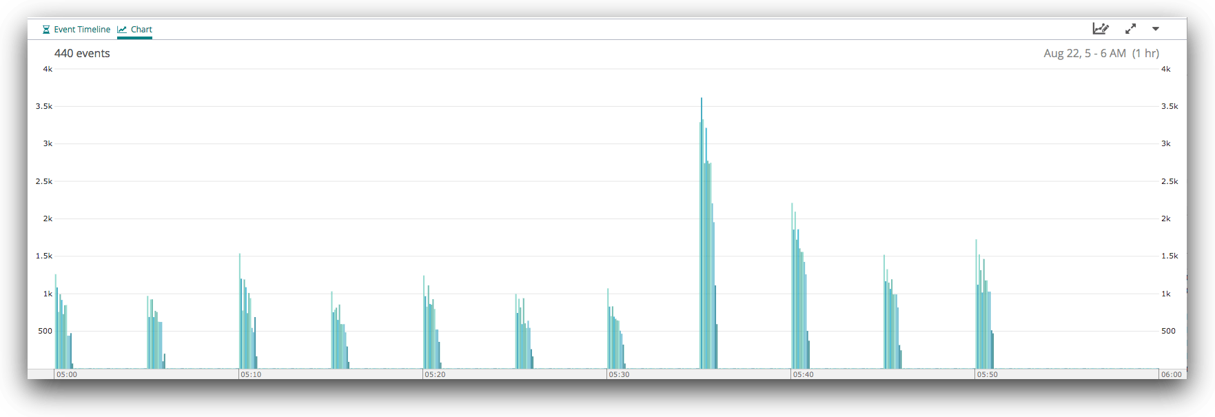
The obvious first thing to look at is how fast we are indexing into each shard. If we graph the sum of the ips (indexing requests per second) values for each shard, we get the following graph:

Here we can see the spike at 05:35, but we can’t really see whether we have a problematic index or shard. If we drill down on the spike at 05:35, we see this:

Each line here represents a single shard. All of our index names end in a six-digit hex ID. From this, we can see that:

1. Out total indexing rate across all shards is about 30,000 events/second.
2. We’re indexing about 8,000 events/second into all of the other shards in the system for which we don’t have details here.
3. Shard 1 of the 34675d index is being written to at about 560 events/second.
4. The c70794 index has seven shards, all being written to at about 780 events/second, or about 5,500 events/second total for the index.
5. The b928ab index has 10 shards, and all are being written to at about 1,620 events/second for a total of about 16,200 events/second (about half the total indexing load for the cluster).

All of this suggests that the system is performing well. If there was a hot node or shard, you might expect that there would be more variation in these numbers. Maybe one shard would stand out with a higher or lower indexing rate. You might expect, moreover, that every indexing node in the cluster would be working equally hard.

Sadly, that isn’t how Elasticsearch works when you’re indexing in bulk. The overall indexing performance is gated by the slowest node on which you’re indexing. If your bulk requests contain roughly the same number of events for each node, you’ll see exactly what we saw above, which is that each shard is indexing at about the same rate as its peers.

Are our nodes balanced?

So let’s look at exactly the same data, but split by node, rather than by shard.

We’ve switched to an unstacked view here, because it allows us to more easily compare each node to its peers for each time period. There are some fairly obvious differences between the nodes in this cluster, and that those differences are stable over time.

Let’s dive in on the spike at 05:35.

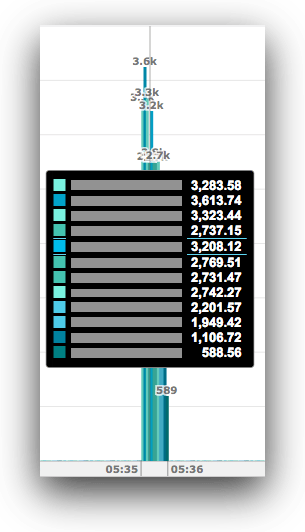
Here we can see the variation between each node pretty clearly—they range from as low as 600 events/second to about 3614. That’s a 6x difference between least and most busy.

Where does this imbalance come from?

We’ve seen some clues in the analysis we did on the shard level performance. The most active index had 10 shards. We know the cluster uses 12 nodes for indexing. This means that two of the 12 nodes simply can’t have a shard for this index and therefore will never receive data for this index. If this was the only index on the cluster, then there is no doubt we’ve misconfigured things: We should be running it with 12 shards.

However, because our clusters are multi-tenant, we have a much more complex “index geometry” problem to deal with. In order to satisfy requirements we have relating to optimal shard size and the maximum age of data in any index, we create indices with widely varying numbers of shards. We rely on the fact that if you size your indices correctly, most shards (irrespective of what index they’re in) should be under about the same indexing load as most other shards. This mostly works out just fine, but because we’re not automatically managing where shards are allocated based on their indexing load, we do see situations like the one we’ve just examined. And even in cases like this, we’re still in pretty good shape because we don’t run our clusters at the limits of their indexing capacity—those same nodes also have to deliver search results.

To give you some context, at the time this Kafka spike occurred, this cluster had 70+ indices and 500+ shards on these 12 nodes. This puts it about in the middle of the pack compared to our other clusters.

Summary

Hopefully you’ve seen the value we can get from our Kafka, writer, and Elasticsearch monitoring. Using this monitoring, we can:

• Quickly, visually identify and deal with major problems in our Elasticsearch clusters
• Understand how (and how well) the system recovers from minor problems
• Understand the normal behavior of the system at a deeper level

The goal in any distributed system is to share the workload as evenly as possible across all available resources. As we saw when we looked at the node breakdown above, that theory doesn’t always map to reality. But only by understanding the details of what happens in reality can we tune the system to get closer to the ideal.

When I started this series, I was hoping to be able to show you a worst-case scenario, with a clear and obvious indexing hotspot that was significantly degrading our cluster performance for 10+ minutes. However, the last such incident happened long enough ago that the logs have been expired from our systems. When it happened, we used the shard-level data to identify the offending index, and replaced it with a new index with more shards.

The only realist way to run complex distributed systems is with automated management, which must be based on the actual behavior of the system. Over time, incidents like this have helped us to identify edge-cases in our automated index management and to gain the capability to detect and preemptively solve them.

I hope that this look into “logfooding” at Loggly has given you some ideas that you can apply to your own systems. For me, the most important takeaway is that the sooner you start collecting this type of data, the better off you will be. It’s only by using the data directly that you will learn its true value. So what are you waiting for?

Related Articles:

How to monitor Elasticsearch performance like a pro

Monitoring Elasticsearch with structured JSON

9 tips on ElasticSearch configuration for high performance

Scaling Elasticsearch for Multi-Tenant, Multi-Cluster

Now that you’ve learned how to visualize a big data pipeline, signup for a FREE no-credit card required Loggly Trial and start to analyze and visualize your data to answer key questions, track SLA compliance, and spot trends. Loggly simplifies investigation and KPI reporting.

>> Signup Now for a Free Loggly Trial

The Loggly and SolarWinds trademarks, service marks, and logos are the exclusive property of SolarWinds Worldwide, LLC or its affiliates. All other trademarks are the property of their respective owners.